Introduction to event studies
How event studies use stock prices to quantify the impact of corporate, regulatory, and macro events.
An event study measures how an event moved a stock's price by comparing the returns it actually earned to the returns you would have expected without the event. In short: estimate a normal-return model (usually the market model) over a pre-event window, take the abnormal return as actual minus expected during the event window, cumulate it into the CAR and average across firms into the AAR and CAAR, then test whether those differ from zero. This page walks through each step, and you can run the whole pipeline free in ARC.
What is an event study?
An event study is a statistical method that measures the impact of a specific event (for example an acquisition announcement, an earnings surprise, or a regulatory ruling) on the value of a firm by examining how its stock price behaves around the event date. The method compares the returns actually observed near the event with the returns that would have been expected in the absence of the event, and attributes the difference (the abnormal return) to the event itself.
The approach rests on an efficiency premise. Under the semi-strong form of the efficient-market hypothesis (Fama, Fisher, Jensen, and Roll, 1969), security prices impound new public information quickly, so the effect of an event is reflected in prices almost immediately. Because prices adjust fast, a relatively short window around the event is enough to capture the event's full economic value: the abnormal return inside that window is, in effect, the market's real-time valuation of the news. Note that this is a working assumption rather than an established fact. A persistent, systematically non-zero abnormal return after an event is itself evidence against market efficiency, so every event study is simultaneously a measure of the event's impact and a joint test of the assumed return model and market efficiency (Kothari and Warner, 2007).
The methodology is most commonly applied to stock returns, but the same logic extends to other market data: abnormal trading volume and abnormal volatility studies (Beaver, 1968; Patell, 1976) ask whether an event moved trading activity or price dispersion rather than the price level.
A short history
The technique has a long lineage. Dolley (1933) is widely regarded as the first event study, examining the price effects of 95 stock splits. The modern, statistically rigorous form was established by Ball and Brown (1968) on earnings announcements and by Fama, Fisher, Jensen, and Roll (1969), the first direct test of market efficiency. Brown and Warner (1980, 1985) provided the simulation evidence validating the test statistics in monthly and daily data, and MacKinlay (1997) together with Campbell, Lo, and MacKinlay (1997) are the standard methodological references.
When event studies are used
Event studies are used across finance, accounting, and law and economics wherever a discrete, dateable event is expected to change a firm's value. Typical applications include:
- Mergers and acquisitions announcements (effects on acquirer and target).
- Earnings surprises and guidance revisions.
- Dividend initiations, cuts, and share-buyback announcements.
- Regulatory decisions and legal rulings (and, relatedly, damages estimation in litigation).
- Product launches, drug approvals, and recalls.
- Macroeconomic and policy shocks (rate decisions, sanctions, elections).
Two horizons are worth distinguishing. Short-horizon studies (a few days around the announcement) are statistically reliable, and the choice of return model rarely changes the conclusion (Kothari and Warner, 2007). Long-horizon inference (months or years) is, in the authors' word, "treacherous," because model misspecification compounds over time. Long horizons are therefore usually measured with buy-and-hold abnormal returns, $BHAR = \prod_t (1+R_{i,t}) - \prod_t (1+R_{m,t})$, rather than the cumulative measures introduced below.
The event study timeline
Every event study is organized around two non-overlapping periods on a timeline indexed relative to the event. Let the event date be $\tau = 0$. The estimation window runs from $T_0$ to $T_1$ before the event and is used to learn what "normal" returns look like for the firm. The event window runs from $T_1+1$ to $T_2$ around $\tau = 0$ and is where abnormal returns are measured. An optional post-event window ($T_2+1$ to $T_3$) can be added to study drift.
</text><text x='40' y='118' font-family='sans-serif' font-size='11' text-anchor='middle' fill='%23334155'>T0</text><text x='290' y='118' font-family='sans-serif' font-size='11' text-anchor='middle' fill='%23334155'>T1</text><text x='450' y='118' font-family='sans-serif' font-size='11' text-anchor='middle' fill='%23334155'>T2</text><text x='600' y='118' font-family='sans-serif' font-size='11' text-anchor='middle' fill='%23334155'>T3</text></svg>)
Source: Own illustration after MacKinlay (1997).
The estimation window must precede, and not overlap, the event window. The parameters that define normal returns (for the market model below, $\alpha$ and $\beta$) are fit by ordinary least squares on the estimation window on the assumption that it contains only ordinary, event-free return behavior. If event-window returns leaked into the estimation sample, the normal-return benchmark would be contaminated and the abnormal returns biased. Event windows are usually short and symmetric around $\tau = 0$, but the concrete lengths to choose (and the empirical evidence behind them) are a procedural decision covered in the guide to choosing estimation and event window lengths.
Abnormal returns
Return event studies quantify an event's economic impact in so-called abnormal returns. The abnormal return is calculated by deducting the return that would have been realized if the analyzed event had not taken place (the normal, or expected, return) from the actual return of the stock. Formally, the realized return decomposes into a normal component and an abnormal component, $R_{i,t} = K_{i,t} + e_{i,t}$, where $K_{i,t}$ is the expected return and $e_{i,t} = R_{i,t} - K_{i,t}$ is the abnormal return, a direct measure of the unexpected change in shareholder wealth associated with the event (Kothari and Warner, 2007).
While the actual return can be empirically observed, the normal return must be estimated. For this, the event study methodology makes use of expected return models, which are also common to other areas of finance research. As a concrete intuition: if on the announcement day a stock returns +5% while the chosen model predicts a normal return of +1%, the abnormal return is +4%, the part of the move the model cannot explain by ordinary market movement.
The market model
The market model is the most frequently used expected return model in event studies. It builds on the actual returns of a reference market and the correlation of the firm's stock with that market. Equation (1) describes the model formally. The abnormal return on a distinct day within the event window represents the difference between the actual stock return ($R_{i,t}$) on that day and the normal return, which is predicted from two inputs: the typical relationship between the firm's stock and its reference index (expressed by the $\alpha_i$ and $\beta_i$ parameters), and the actual reference market return ($R_{m,t}$).
$$AR_{i,t}=R_{i,t}-(\alpha_i+\beta_i R_{m,t}) \tag{1}$$
The parameters $\alpha_i$ and $\beta_i$ are not assumed; they are estimated by ordinary least squares over the estimation window that precedes and does not overlap the event window. In estimation form the model is written $R_{i,t} = \alpha_i + \beta_i R_{m,t} + \varepsilon_{i,t}$ with $E[\varepsilon_{i,t}] = 0$ and $\mathrm{Var}(\varepsilon_{i,t}) = \sigma^2_{\varepsilon}$. The fitted parameters are then projected onto the event window to produce the predicted normal return, and the residual relative to the actual return is the abnormal return in Equation (1).
The market model is one choice among several, and each is treated in full on the expected return models page:
- The constant-mean (mean-adjusted) model sets the normal return to the average estimation-window return, $AR_{i,t} = R_{i,t} - \bar{R}_i$.
- The market-adjusted model imposes $\alpha_i = 0$ and $\beta_i = 1$ so that $AR_{i,t} = R_{i,t} - R_{m,t}$ and needs no estimation window.
- The CAPM prices normal return off a single market risk factor and a risk-free rate.
- The Fama-French three- and five-factor models add size, value, profitability, and investment factors to the market factor.
- The Carhart four-factor model augments the three-factor model with a momentum factor.
A practical example
To make the calculation concrete, consider a single firm over a five-day event window around an announcement (days $-2$ to $+2$). The normal return is predicted by the chosen model, and the abnormal return is the actual return minus the normal return. Summing the daily abnormal returns gives the cumulative abnormal return over the window.
| Relative day | Actual return | Normal return | Abnormal return (AR) |
|---|---|---|---|
| -2 | +0.4% | +0.3% | +0.1% |
| -1 | +0.6% | +0.2% | +0.4% |
| 0 | +5.0% | +1.0% | +4.0% |
| +1 | +0.9% | +0.4% | +0.5% |
| +2 | +0.1% | +0.3% | -0.2% |
| CAR(-2,+2) | +4.8% |
The cumulative abnormal return of +4.8% summarizes the market's reaction over the window, concentrated on the event day. To translate a percentage into a dollar wealth effect, multiply by the firm's market value of equity at the event: $\Delta W = CAR \times \text{(market value of equity)}$. For a firm worth USD 10 billion, a +4.8% CAR corresponds to roughly USD 480 million of created shareholder value. (The numbers above are illustrative.)
Average and cumulative abnormal returns (AAR, CAR, CAAR)
Abnormal returns can be aggregated along two distinct axes. Across time, the daily abnormal returns of a single firm are summed into a cumulative abnormal return (CAR). Across firms, the abnormal returns of many events on the same relative day are averaged into an average abnormal return (AAR). Doing both yields the cumulative average abnormal return (CAAR). Keeping these two axes separate is the key to reading the formulas below.
The average abnormal return is the cross-sectional mean abnormal return on a single relative day $t$, taken across the $N$ firms in the sample. It is therefore indexed by $t$, as shown in Equation (2) (Kothari and Warner, 2007).
$$AAR_t= \frac{1}{N} \sum_{i=1}^{N}AR_{i,t} \tag{2}$$
To measure the total impact of an event over a particular period (the event window) for a single firm, one adds up that firm's individual abnormal returns to create a cumulative abnormal return. Equation (3) shows this for one event $i$; the firm index $i$ on the summand makes explicit that this is a per-firm quantity.
$$CAR_i(t_1,t_2)=\sum_{t=t_1}^{t_2} AR_{i,t} \tag{3}$$
Figure 2 plots the CAR values of two different corporate event types, FDA approvals and the issuance of special dividends, as they change when the event window is gradually extended. The figure suggests that the capital market perceives both event types as good news.
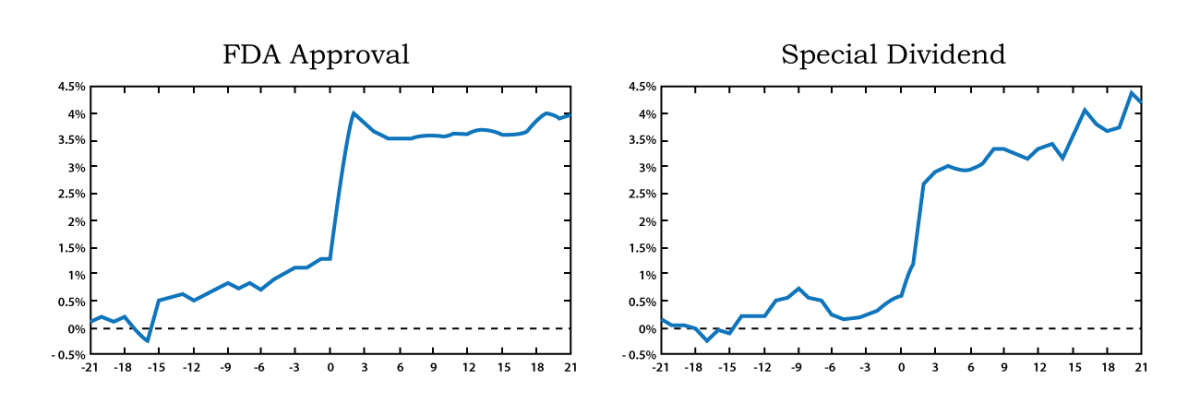
Source: Adapted from Neuhierl et al. (2011: 48); published as Neuhierl, Scherbina, and Schlusche (2013).
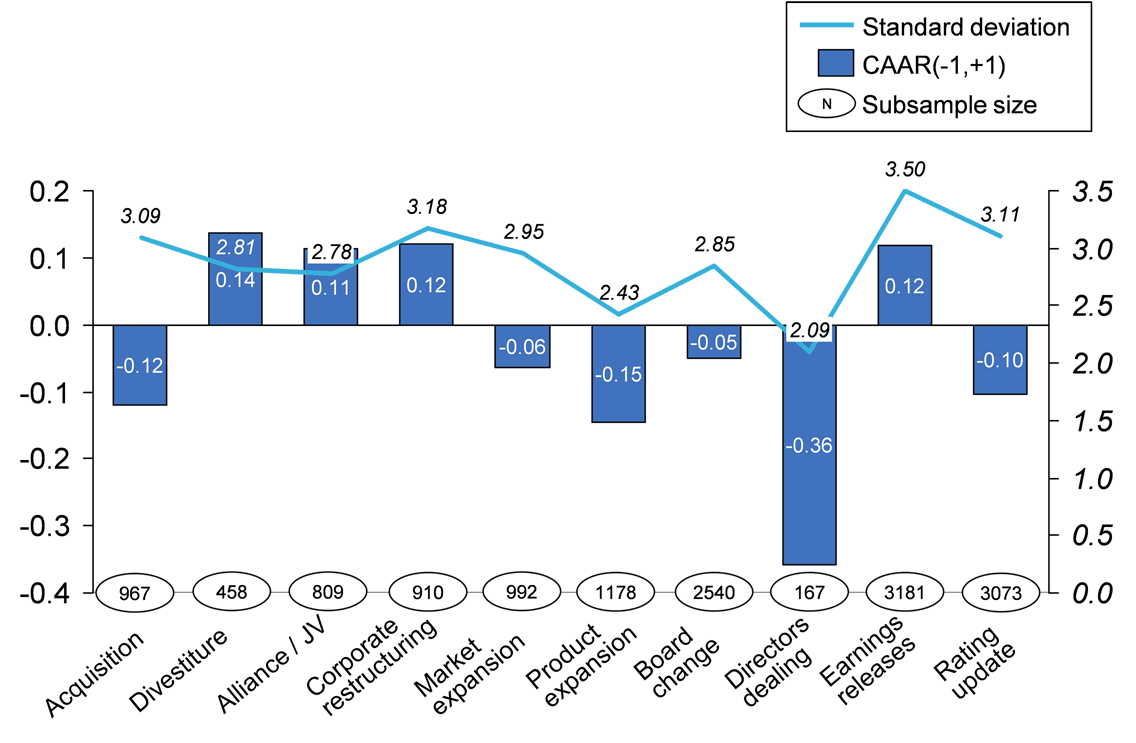
In a sample event study that holds multiple observations of an event type (for example acquisitions), one can further calculate cumulative average abnormal returns (CAARs), which represent the mean cumulative response across the sample of identical events. Equation (4) shows the formal equation for CAARs, using the same sample-size symbol $N$ as Equation (2). Figure 3 illustrates CAARs and their standard deviations from a ten-year study of the global insurance industry (Schimmer, 2012). The presented CAARs represent the average stock market responses (in percent) to press releases describing different types of corporate decisions.
$$CAAR(t_1,t_2)= \frac{1}{N} \sum_{i=1}^{N}CAR_i(t_1,t_2) \tag{4}$$
The two aggregation orders coincide: averaging the firm-level CARs is identical to summing the average abnormal returns over time, $CAAR(t_1,t_2) = \frac{1}{N}\sum_{i=1}^{N} CAR_i(t_1,t_2) = \sum_{t=t_1}^{t_2} AAR_t$. In short: AR is one firm on one day, $CAR_i$ is one firm summed over time, $AAR_t$ is many firms averaged on one day, and CAAR is both.
Source: Own Illustration
Once you understand how abnormal returns are defined and aggregated, the next step is procedural. For the full recipe, see how to run an event study, step by step.
Is the result significant?
A CAR or CAAR is a point estimate, and its magnitude alone is not evidence. Each is tested against the null hypothesis that the mean abnormal return is zero ($H_0: E(AR) = 0$, or $H_0: E(CAAR) = 0$). The simplest test is a parametric t-test that divides the abnormal return by its estimated standard deviation (the estimation-window root mean squared error), which relies on the abnormal returns being approximately normally distributed. Under the market model the relevant variances are $\mathrm{Var}(CAR_i) = (t_2 - t_1 + 1)\,\sigma^2_{\varepsilon}$ and, for $N$ independent events, $\mathrm{Var}(CAAR) = \mathrm{Var}(CAR_i)/N$.
Because the plain t-test is sensitive to non-normality and to the variance an event can induce, more robust statistics are common. Standardized tests such as Patell (1976) and the standardized cross-sectional test of Boehmer, Musumeci, and Poulsen (1991) correct for event-induced variance, and non-parametric tests such as the sign test and the Corrado (1989) rank test drop the normality assumption entirely. Our significance tests page documents the full parametric and non-parametric battery.
A closing validity note: the abnormal return isolates the event only if no other material news (earnings, M&A, lawsuits) occurs inside the window, so confounding observations must be screened out; the screening procedure is set out on the Application Blueprint. Data choices also matter at the margin (daily versus monthly returns, simple versus log returns, and the choice of reference index), and the Blueprint's data choices section gives the practical guidance.
Ready to run one?
This page covers what an event study is and how abnormal returns are defined, aggregated, and tested. To carry the method through from event-date identification and window selection to publication-ready test statistics, follow the Application Blueprint, the step-by-step companion to this introduction.
In addition to the above introduction, you may find the subsequent third-party video on YouTube helpful.
References and additional links
Neuhierl, A., Scherbina, A. and Schlusche, B. 2011. 'Market reaction to corporate press releases'. Available at SSRN: http://ssrn.com/abstract=1556532. Published as 'Market Reaction to Corporate Press Releases', Journal of Financial and Quantitative Analysis 48 (4): 1207-1240 (2013).
Schimmer, M. 2012. Competitive dynamics in the global insurance industry: Strategic groups, competitive moves, and firm performance. Wiesbaden: SpringerGabler.
References
- Ball, R., and P. Brown. 1968. "An Empirical Evaluation of Accounting Income Numbers." Journal of Accounting Research 6 (2): 159-178. https://doi.org/10.2307/2490232
- Beaver, W. H. 1968. "The Information Content of Annual Earnings Announcements." Journal of Accounting Research 6 (Supplement): 67-92. https://doi.org/10.2307/2490070
- Boehmer, E., J. Musumeci, and A. B. Poulsen. 1991. "Event-Study Methodology Under Conditions of Event-Induced Variance." Journal of Financial Economics 30 (2): 253-272. https://doi.org/10.1016/0304-405X(91)90032-F
- Brown, S. J., and J. B. Warner. 1980. "Measuring Security Price Performance." Journal of Financial Economics 8 (3): 205-258. https://doi.org/10.1016/0304-405X(80)90002-1
- Brown, S. J., and J. B. Warner. 1985. "Using Daily Stock Returns: The Case of Event Studies." Journal of Financial Economics 14 (1): 3-31. https://doi.org/10.1016/0304-405X(85)90042-X
- Campbell, J. Y., A. W. Lo, and A. C. MacKinlay. 1997. The Econometrics of Financial Markets, ch. 4. Princeton, NJ: Princeton University Press.
- Corrado, C. J. 1989. "A Nonparametric Test for Abnormal Security-Price Performance in Event Studies." Journal of Financial Economics 23 (2): 385-395. https://doi.org/10.1016/0304-405X(89)90064-0
- Dolley, J. C. 1933. "Characteristics and Procedure of Common Stock Split-Ups." Harvard Business Review 11 (3): 316-326.
- Fama, E. F., L. Fisher, M. C. Jensen, and R. Roll. 1969. "The Adjustment of Stock Prices to New Information." International Economic Review 10 (1): 1-21. https://doi.org/10.2307/2525569
- Kothari, S. P., and J. B. Warner. 2007. "Econometrics of Event Studies." In Handbook of Corporate Finance, Vol. 1, edited by B. E. Eckbo, ch. 1, 3-36. Amsterdam: Elsevier. https://doi.org/10.1016/B978-0-444-53265-7.50015-9
- MacKinlay, A. C. 1997. "Event Studies in Economics and Finance." Journal of Economic Literature 35 (1): 13-39. https://www.jstor.org/stable/2729691
- Neuhierl, A., A. Scherbina, and B. Schlusche. 2013. "Market Reaction to Corporate Press Releases." Journal of Financial and Quantitative Analysis 48 (4): 1207-1240. https://doi.org/10.1017/S0022109013000409
- Patell, J. M. 1976. "Corporate Forecasts of Earnings Per Share and Stock Price Behavior: Empirical Tests." Journal of Accounting Research 14 (2): 246-276. https://doi.org/10.2307/2490543
- Schimmer, M. 2012. "Essays on competitive dynamics: Strategic groups, competitive moves and performance within the global insurance industry." Dissertation, University of St. Gallen, St. Gallen. https://doi.org/10.1007/978-3-8349-3992-0
See the full bibliography for all sources cited across the site.